Microarray Tour, 2002, Laura L. Mays Hoopes, Pomona College
Stanford Microarray Database, 7/11/02-7/12/02
At Stanford, I was was graciously hosted by Dr. Barbara Dunn, who came to one of the ASCB genome workshops featuring GCAT. I arrived during consolidation of 96 well plates to 384 well plates in preparation for printing microarray slides of yeast ORFs. Barbara Dunn told me that to make the DNA for the arrays, she used pairs of primers that bracket each yeast ORF, purchased from Research Genetics. She said that the newer ones Research Genetics sells will bracket an approximately 1kb part of each ORF that does not overlap the sequence of another ORF wherever possible. But, the Stanford slides GCAT obtained in 2000-2001 were made with PCR products of the whole ORFs similar to those she was about to print again. She received the primers in deep (200 ul) 96 well plates. From these, she aliquots 5 ul of each primer into the well for the ORF, and when all are ready for the run, she makes a master mix of the template DNA, the Taq polymerase, nucleotides, and buffer components and aliquots the mix to each well with the individual primer set in each well. She said she runs the PCR reactions for 800 ORFs at once, and makes 3 PCR runs a day for about three days to get them all done. Each has gel electrophoresis done as a quality control, to make sure the product size is correct.
Barbara and Cheryl inspecting the PCR products in 96 well plates
Cheryl and Elena from the microrarray core facility were working on the arraying process. Barbara and I worked with her for a while, opening and placing onto the correct location on the robot platform 4 boxes of 96 pipet tips, 4 of the PCR-product-96 well plates, and 4 392 well plates with very tiny holes into which the products were being transferred by the robotic system. The robotic system loaded the tips from one box, sucked up 4 * 23 ul from each of the PCR product wells, and then dispensed a 23 ul aliquot into the correct well of each of the tiny 392 well plates. The process was making 4 identical 392 well plates. In each set of four rounds of dipping into the 96 well plate wells, a square block of wells in the 392 well plate would be filled. The order would be top left, top right, bottom right, bottom left (clockwise around a circular path). Then the robot would move on to the next block to the right of the square it had just finished. At the end of a row, it would move to the left end of the second row down, skipping the row that had been filled as the Śbottomą in the blocks it just completed. Cheryl said that there would be 4000 microarray slides printed from the 4 sets of 392 well plates we worked on.
Cheryl placing a 96 well plate onto the robot. The pipet tips are in the aqua boxes to the left and the 384 well plates are in the column to the right of where she is working.
Later, we watched Ashley set up his Śboosterą fluorescent cDNA synthesis reactions and post-process his microarray slides for use. Barbara had post-processed all of the Stanford slides for us, and because ISB uses long oligonucleotides rather than double stranded PCR products, and uses something other than polylysine as the slide coating to bind the printed DNA, the post-processing Stanford does is quite different from the protocol we got from ISB. First, the slides were left 15 minutes at room temperature with array side down over room temperature water in a hydrator tray with a top. During this step, the spots became clearly visible and were supposed to Ślook shinyą. Ashley said he uses time because he cannot see what is meant by shiny. After the 15 minutes, the slides were reversed and placed on a 70 degree heat block (the block is turned upside down so the holes face down and a flat plate faces up). It is only left on the block a few seconds until it looks dry. Then, the slide is placed in a rack and it is post processed using 2 methyl pyrollidone in which is dissolved succinic anyhydride. Then the arrays in a rack are plunged into sodium borate, treated with hot water, and dried with ethanol. Finally they are spun dry.
The hybridization chambers used are metal two piece chambers held together with screws, that were made to order for the lab. They have a well for hydration water to be added to prevent excessive drying during the hybridization at 65 degrees for 16 hours. I saw that others in the group were using the Corning microarray hybridization chambers that are two piece plastic holders with two well for hydration water, held together with two metal sliding clamps. The Corning ones are not light-tight, so people said that they had to make sure that light would not hit the chamber during hybridization. The hybridization buffer used does not contain formamide, thus the high temperature is necessary. Ashley says he uses a wider and longer coverslip to help keep the probe from becoming unevenly distributed. Barbara said that she had seen a number of microarrays where it looked like the probe was more concentrated around the edges than in the center of the array. They mentioned the possibility of using lifter cover glasses, which would hold more volume under them over the array and not be drawn down too tight on the center of the array. These would have to be special ordered, since they are not generally available.
On Friday, 7/12/02, Barbara and I worked a while on inputting some GCAT data into the SMD. She explained to me that if the image that comes from the two tif files is not what is wanted, it is possible for the account owner, Malcolm in our case, to replace it with an BITMAP image that we prefer, saved in Scanalyze with two colors. But it is necessary for the replacement image to be exactly the same size and orientation as the original for the SAG file we provided, to hit our spots with the grid boxes. She and I made new images for some of my recent data from Jessica Brownąs senior thesis, and planned to ask Malcolm to upload them using his password.
During the late morning, there was a gene expression group presentation by a graduate student each from David Botsteinąs lab and Pat Brownąs labs. Maitreya Dunham talked about characterizing gene rearrangements occurring during experimental evolution. Caroline Uhlik than talked about identifying and mapping genetic variations in genomic expression programs, via a cross between two strains of yeast. Both engendered a good deal of discussion, with Pat Brownąs comments being of particular interest.
Later, Barbara and I met with Gavin Sherlock, one of the curators of the Stanford Genome Database. One question I asked him was about how much replication is enough for believable data. Both he and Barbara thought 3 independent arrays was right for projects like comparing two states or comparing a mutant and a wild type. However, they had some interesting differences of opinion about timecourses with multiple points. Gavin thought that one run per point with more points, but two separate series of time points generated by different methods would be the most convincing. He mentioned the use of alpha arrest/release and temperature sensitive cdc15 mutant block/release as two ways that the cell cycle was studied, and that using these two, those genes with similar responses popped out without any need to worry about duplicates. But because time zero point is the basis for the rest, it should always be replicated. Barbara thought at least 2 arrays per point would be required, even in a time series. They both thought that replicates should be with separate RNA preparations, not equivalent to the two spots next to each other on the ISB chips. The chips Barbara is printing will have two complete microarrays per slide, and she could potentially hybridize them with different probes at the same time if she wishes.
Another topic that came up in that meeting was quality control of RNA. Both Barbara and Gavin thought that a gel should be run on the total RNA; ideally if quantities permit, also on the mRNA and a Northern for sizes of specific mRNAs. Neither of them usually does a gel on mRNA. The quantities of RNA per array are pretty standard for Stanford researchers: 20 ug of total RNA or 2 ug of mRNA. I asked about the lack of correspondence of these numbers since mRNA yields we get are more like 1-2% of total rather than 10%, and they said they were empirically chosen to maximize signal and minimize background. They thought that using 100 ug of total RNA would give a lot more background than would be wanted.
We had missed seeing the test prints made of the PCR products, but Elena was laying out 250 slides on the microarray printer for a print in the clean room, and we were able to watch and to talk with her a bit through the glass porthole in the door. She said that she had printed one slide with multiple redottings of the same samples and one exactly as the real run would be done, with only two dottings per sample. Both looked very good under the dissecting microscope, so she would be ready to start printing Barbaraąs arrays on Monday. It will take her 8 working days to print the 4000 arrays. They donąt like to leave the arrays long during printing. The microarray printer looks a lot like the robot used to consolidate the two kinds of plates together; it simply picks up from the plate and dots onto the slide repeatedly in a known pattern. I asked Barbara why the dots are visible before post processing but not after, and she said that it is because of the salts in the sample that are washed off during the post processing.
We dropped in to touch base with one of Barbaraąs colleagues who was involved in preparing the DNA for the microarray printing, to talk with him about the resolution of a problem that had been encountered. The PCR products in their 96 well plates had been ethanol precipitated but some of them had been topped with a different kind of plastic cover that partially dissolved in the ethanol and may sticky and stringy messes in some of the tubes. A great deal of care had to be exercised by Cheryl in the placing of these particular samples into the 392 well plates so that none of the tips would be clogged and none of the apparatus would stick together when it should be separating after interacting. Luckily, the fatal covers had only been used on a few of the plates. After assuring him that the process went well and so had the test print earlier in that day, he talked about control spots. Interestingly, he and Barbara agreed that they usually do not look at the data for the control spots on the arrays. However, he puts some RNA transcribed in vitro from Bacillus DNA into each sample and puts specific Bacillus DNA dots on his arrays; this helps in case of different amounts of RNA in different samples before cDNA synthesis. They discussed a similar type of control using a different bacterium that is currently available through the core facility printing Barbaraąs new arrays, and she is going to think about using this control.
ISB July25-27, 2002
Institute for Systems Biology, Seattle
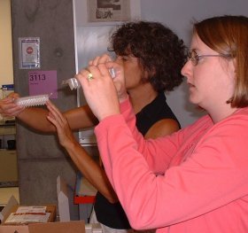
I found Institute for Systems Biology near the North shore of Lake Union, just to the west of the University of Washington campus in Seattle. I parked in the parking garage and went upstairs to the lobby. The receptionist paged Dr. Krassen Dimitrov, the Director of the Microarray facility and he came out, welcomed me, and gave me a tour of the ground floor. We talked a bit about methods of microarray use and data analysis. Then he introduced me to Allison, Bruz, Meredith, and Steve who work with him on microarrays. Allison had obtained some yeast RNA for me to label and hybridize and gave me protocols to follow. She showed me where the chemicals and supplies I would need were stored. Also, I was able to follow Meredith, who was labeling some cDNA from monkey brain RNA and was about 10 minutes ahead of me all the way through. First, we spiked each sample with a characteristic pair of RNAs that would hybridize with particular control spots on the microarrays. Then, I annealed each 50 ug of total RNA with oligo dT. Then, I added reverse transcriptase buffer, DTT, deoxyribonucleotide mixture with low dCTP, either Cy3 dCTP or Cy5 dCTP, and Superspcript II reverse transcriptase. The prealiquotted dyes were stored in dark red microfuge tubes to protect them from light during storage. After mixing the components of the reverse transcription reactions, I incubated at 42 degrees for 2 hours.
During that time, I met with Bruz to hear about the methods used for microarray data analysis. He showed me how they set up the scanner to read at a level where no spot reaches or exceeds the maximum reading, and then also at a level where all spots are high and some are maxed out. The average relationship between spot intensities can be used to calculate what the real value for a maxed out spot should be, and then that is used to correct the Śhighą scans. They use spot finding software that allows two color scans at two intensities (all four scans) to be stacked and the spots defined for the whole stack.
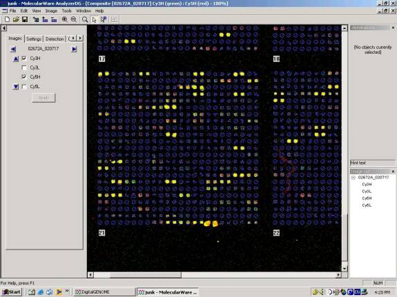
Example of some good data from a yeast microarray.
Then he showed me the kind of software that they use to see whether or not a spot has changed due to the conditions used. It is available on the ISB web site, using a combination of VERA and SAM software programs. It analyzes all the replicates of a gene, both the duplicates on each array and replicate arrays, and it provides a statistical evaluation of the change observed in the form of a lambda score. Bruz said that unchanged spots would have scores from about -0.80 to 1.2. The analysis does a log transform on the data, so a minus would indicate the expression decreased while a plus that it increased. A lambda of 2 is considered a strong change. I asked about replication, and Bruz told me that they recommend and ideal data set with 4 microarrays (each with duplicate spots and duplicate supergrids) with reversed colors. Two would have red on one type of sample and the other two would have red dye on the opposite type of sample. Dye reversal is very important according to Bruz. He said they could see curvature in the absorbance/absorbance plots for the data with dye in one direction, and the opposite curvature with dye in the other direction, balancing out the dye effect when both were included equally in the data. He showed me data indicating that even in same sample hybridizations, there is a clear dye effect.
After the 2 hour incubation was finished, I treated with RNases to get rid of the RNA, leaving just the dye-labeled cDNA, then cleaned up the product using Qiagen PCR purification columns. Then we put the sample into a 384 well plate absorbance reader with a special plastic plate that enabled readings at 260, 550, and 650nm. My samples had decent reading for the 260 nm absorbance (about .3) but very low readings for each dye. Allison told me that 0.1 -.2 or more was a reasonable reading for those, and the highest I had was only 0.9, while some were .03. So, she encouraged me to use the entire sample for each slide. I had a choice of either pooling the two samples for each slide together before SpeedVac drying or after. I chose before, and as a result had to wait 1.5 hours for them to dry down to 1-2 ul. I recommend pooling them after drying down! At this point, I was excited to see that there was a little color in each of my samples, possibly indicating that the cDNA had been successfully labeled.
While the drying occurred, we post-processed the slides to be used. We steamed them briefly, with the spot side down (10 seconds or so) over a 1 liter beaker of boiling water. When they looked like the spots were hydrated, we plopped them, with spots on the top side, onto a 90 degree hot plate for 30 seconds. Then we resteamed and dried on the hot plate for 1 minute. This step redistributes the oligos more evenly onto the spots, so you donąt get rings around your spots, or fried egg effects. Next we placed each slide in a 50 ml tube of 3 x SSC, 0.1 % SDS (we reused tubes of this that had already been used previously), screwed the top on tight, and placed them horizontally on a tiny orbital shaker. After 30 minutes, we took them out, dipped them briefly in deionized water, and blew them dry with compressed air. They were stored in slide box until used. This procedure is much easier and less toxic than the one used at Stanford because oligonucleotides 70 nucleotides long are used here rather than double stranded PCR products of the whole ORF. They explained that these would be more specific, avoiding problems with overlapping genes that are transcribed from opposite strands of DNA, which are fairly common in yeast. Of course, they preclude the use of Alexa-dye-coupled mRNA since they are the sense strand, similar to the mRNA and thus will not hybridize with it. The coverslips had been previously cleaned with water and ethanol and dried; these were stored in a 50 ml screwcap centrifuge tube until used.
To set up the hybrization, I added the hybridization buffer to the 1-2 ul samples from the Speed Vac. They use the DIG Easy Hyb buffer with added denatured, sheared salmon sperm DNA, tRNA, and poly A. This buffer is proprietary with Roche, but they indicate that it is denaturing (similar to formamide buffers) but contains less toxic compounds than formamide. We mixed the samples with the hybridization buffer, then denatured the mixed probe in hybridization buffer for 2 minutes at 95 degrees. Then we quick cooled them and spun them down to break bubbles, then placed the liquid on one end of the slide. We touched a coverslip to it, then balanced it on a syringe needle with the beveled side up and slid the needle back slowly to lower the coverslip onto the slide without trapping bubbles. This was hard for me; Allison did it very well though. Then each slide was placed in a Corning hybridization chamber with 10 ul of water in each of its wells, and sealed up. The chambers were immersed in a waterbath for hybrization. For oligonucleotide slides in this buffer, the ISB group starts the hybridization at 45 degrees and sets the thermal programmer to 37, so the cDNA goes through an annealing process as the temperature cools. They incubate at 37 degrees overnight.
The next morning, Bruz was washing the slides that Meredith had set up the previous day so I was able to follow along with him. They do all wash steps in 50 ml screwcap centrifuge tubes except for the last dip step, which uses a larger volume. Before starting they warm wash solutions for two of the steps to 55 degrees. Step 1 is to immerse the slide, with the engraved label end up, in 55 degree 1 x SSC, 0.1% SDS in a 50 ml tube filled to the brim. This sits upright for about a minute, then the coverslip falls off. With a clean forceps, the coverslip is removed and discarded, being careful not to scratch the array. Then the top is screwed on tight and the tube is placed on its side on the tiny orbital shaker for 5 minutes (at room temp, although the tubes still felt warm when done). Bruz explained to me that it is essential NEVER TO LET THE SLIDE DRY AT ALL DURING THE WASHES, KEEP IT MAXIMALLY WET. Otherwise, you get background smears that cannot be washed off at all. So, keep the slide immersed and instantly move it from one solution to the next, donąt try to quantitatively remove the previous solution during the transfer.
The first wash is dumped out (into the sink; I had heart failure thinking the slides would fall out, but they did not). The second wash, 0.1x SSC, 0.1% SDS at room temperature, is immediately added to fill each tube and the tube is returned to the shaker for 5 minutes. Wash 2 is dumped and replaced immediately with 55 degree 0.5x SSC, then returned to the shaker for 5 minutes. The third wash is dumped and replaced with 0.1 x SSC at room temperature. The tube is left upright and inverted two or three times over a 2 minute period. Then, with forceps, the slide is removed from this wash and dipped several times in a container holding about 100 ml of 0.1x SSC at room temperature, then immediately blown dry with air and stored in the dark until read.
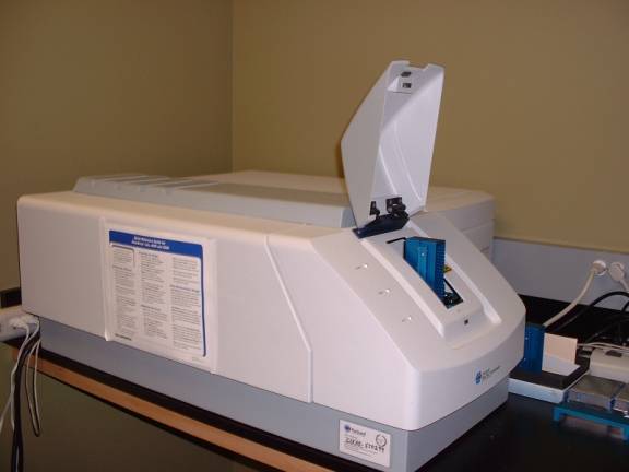
Microarray scanner ready to load with a slide.
Unfortunately, my slides had no signal, so although I saw Bruz attempt to scan them, I could not do any data analysis steps. However, Allison was printing some test microarray spots and I got to see the process. They use Telechem Superamine slides (see ArrayIt.com) so they have no need for polylysine coating on the slides.
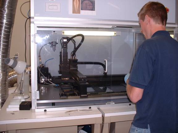
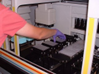
Bruz checking out the operation of the microarray printer. The slides are laid out adjacent to each other and are in the area that resembles a glass plate just to Bruząs left in this picture.
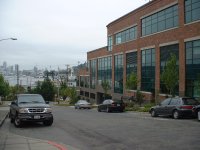
Lake Union and Seattle from ISB
![]()
![]()
![]()
© Copyright 2002 Department of Biology, Davidson College,
Davidson, NC 28035
Send comments, questions, and suggestions to: macampbell@davidson.edu