A Guide to Descriptive Statistics

LAB #7

A Beginner's Guide For Descriptive Statistics

Once you have collected a large set of data, you need to use some descriptive statistics to convey the important aspects of the distribution of your data. Two features of the distribution that you should describe are:
1) the central tendency
2) the spread of your data

Mean
A simple measure of the central tendency of the data is the mean (or average):
mean = sum of all the data ÷ sample size (often called n)

For example, with the data set (1,1,1, 5), n=4, the mean is 8 ÷ 4 = 2.

Range
The simplest measure of the spread of your data is the range which tells you the distance between your most extreme data values, but does not address the issue of how frequent these extreme values are. The formula for calculating the range is:
range = value of maximum data point minus value of minimum data point

For example, with the data set (1,1,1, 5), the range is 5 - 1 = 4.

Variance
The variance of your data is a measure of spread that will take into account both the deviations of your data (away from the mean) and how frequently these deviations occur. For each data point, the mean is subtracted from the data point, and this value is squared.These squared values are added together and divided by either n or n mnus 1. If you sampled an entire population, then you divide by n. If you sampled a subset of a population, you divide by n-1. In our case, we assumed the entire population was sampled. The formula for calculating variance is:

variance = the sum of (each data point minus the mean)²÷ sample size

For example, with the data set (1,1,1, 5): (1-2)² + (1-2)² + (1-2)² +(5-2)² = 12

The variance is 12 ÷ 4 = 3.

Standard Deviation
The standard deviation of your data is the square root of the variance, and therefore it reflects both the deviation from the mean and the frequency of this deviation. Standard deviation is often used instead of the variance because the scale of the variance tends to be larger than the scale of the raw data, while the standard deviation is on the same scale as most of the data. The formula for standard deviation is:

standard deviation = sq root (variance)

For example, with the data set (1,1,1, 5), the standard deviation is the square root of 3 = 1.73

Standard Error of the Mean
The standard error of the mean is another common way to describe the deviation from the mean and the frequency of this deviation but it also takes into account the size of your data set. The formula for standard error is:

standard error = sq root (variance / n) (n= sample size)

For example, with the data set (1,1,1, 5), the standard error is the square root of 3 ÷ 4 = 0.866.

To see why standard error is a useful statistical description, let's consider another data set where the variance was 3 but n = 30.

Standard Error = square root of 3 ÷ 30 = 0.316.

The same variance of 3 gave different standard errors (if n=4: 0.866 versus if n=30: 0.316) due to the difference in sample size. However, if you look closely at standard error and standard deviation, you will notice that standard error has taken the sample size into account twice. In reality, this is statistics at its worst. Standard error is a statistical analysis of one set of data treated as if you had actually repeated the same experiment many times and gotten a range of means. In other words, standard error is a statistical approach that attempts to look at the variance of these imaginary range of means and determine the variance of these means. Many scientists use standard error to make their data look better than it really is. What we would like to be able to say is we are > 95% sure that if we were to repeat a particular experiment another time, the mean value would fall within a certain range. Excel can generate a 95% confidence interval as well.

Excel for Office

W have decided to give you the quick and dirty version that is much easier than older versions of this lab. Once you have obtained results in Excel, you will use Cricket Graph to graph your results. You could use Excel for graphing, but putting error bars in Excel is difficult to do.

1) Enter your data with the times listed down the first column and with your flagella measurements going across in rows.

Save these data: give the file a good name and have the file saved to the Bio111 folder and your section's lab folder. When entering the same number many times, you can save yourself some time with a short cut. Enter the number once, highlight that number, then click and drag the small box in the lower right hand corner to fill as many boxes as you need with the same number.

2) Once all the data are entered, save the file again.

Start a new column called average length and click on the first box:

Click on the Insert menu and select "Function"

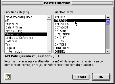
3) You will see a window like the one shown above. Select Statistical and then Average and click on OK. You will get a dialog box like the one below. At the top is the formula for averaging the data entered in boxes B2 through U2. You want to make sure all the boxes that you want to have averaged are within the range you have selected. Do not select A2 sine that has your time values in it. Then click OK.

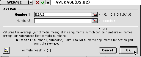
4) When you hit OK, you will see this:

Put your cursor on the box as shown and click and drag down until you reach the 60 minute row. When you let go, all the averages will be calculated.

5) Create a new heading called Standard Deviation:

Click on the box below. Go to the insert menu and

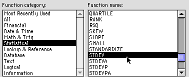
select "Function" Select Statistical and STDEV as shown:

6) You will get another dialog box. Enter the same range as before. In our example, we are using B2- U2 so we would type "B2:U2"

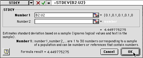
When you click on OK, the value will be entered (probably close to 0). Then click on the lower right hand corner and drag it down to the 60 minute level. This will calculate the standard deviation for all of your averages.

7) Enter a new heading called 95% confidence.

Under this heading click on the next box.

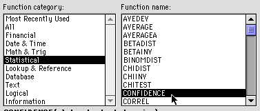
Go to the Insert menu and select "Function" as you did earlier. You will see this dialog window. Select statistical and confidence as shown.

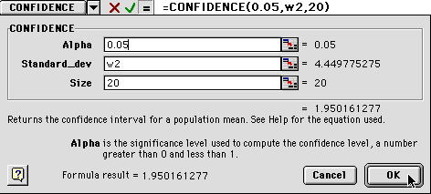
7) Now you will get a new dialog box:

You will need to enter some information:

1) The alpha number is the percentage of confidence you want. Enter 0.05.
2) The Standard_dev is can be obtained by typing in the box location where the first standard deviation was pasted W2.
3) The size is your sample size, or n value. For us it will be 20.

8) When you have done this, you will see something like the dialog box below. Notice that the values are entered in the white boxes, but the numbers are shown to the right, near the cursor in the figure below. The standard deviation has to be greater than zero to calculate the confidence value, but don't worry about this for now.

9) When you click OK, you will get either a number or a "#NUM!". This is Excel's way of telling you that zero is an unacceptable value for standard deviation. Ignore that and drag the box down to calculate all the confidence values through 60 minutes.

After you have obtained all the values, change your "#NUM!" values to zero.

10) You are almost done with Excel. Highlight your data as shown and be careful not to highlight the text above only the number values.

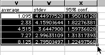
Copy and paste this into Cricket Graph. Now you are ready to quit Excel and use the Cricket Graph directions as found in Appendix A in the back of this manual. You will want to enter time values in the first column under a heading of "time (min)". Then paste your data into the second column. Now graph your averages as a function of time. Then use the 95% confidence values for your error bars.

READ THIS!

After your presentations next week, you will need to address the following issue before you leave lab:

Your group should design next week's experiment, which will be to choose any chemical, product, etc. that you want to test for mutagenicity using the Ames test. By Friday at class the week before the Ames test, bring something YFPM (Your Favorite Potential Mutagen) you've been curious about or have heard "might cause cancer": tobacco, hair dyes, smoked meats, fried bologna, charcoaled hamburger, pesticides, insecticides, rat poison, UV light, caffeine, ethidium bromide, mustard, peanut butter - be creative!

When your read Lab #8 about the Ames test, be sure to think about controls (positive and negative) as well as maybe one or two concentrations of your test chemical. Do your protocol as before: state a hypothesis, how many conditions you are going to test (and thus how many petri plates you will use), and be detailed enough in your outline of procedures so that you know what you are doing.

Table of Contents